In this post, we have explained step-by-step methods regarding the implementation of the Email spam detection and classification using machine learning algorithms in the Python programming language. We have used two supervised machine learning techniques: Naive Bayes and Support Vector Machines (SVM in short). The project implementation is done using the Python programming class concept, to easily manage the code. To view, the complete project report visit the Email spam classification project report. There are separate functions written in the code based on the steps such as:
- Reading and writing CSV files.
- Data Understanding and Data Exploration:
- Generating word cloud using Python wordcloud library
- Data cleaning: Removing punctuation, stop words
- Applying Count Vector Word Embedding Technique
- Applying Naive Bayes and Support Vector Machine (SVM)
- Evaluation: Accuracy and F1 Score, Confusion Matrix, ROC, AUC Curve
We have used three CSV files in the given code. First is the original CSV file for the given dataset and the other two are processed CSV files. You can download all the given files from the links given below.
Download links for the email spam classification dataset
To download the complete code visit the link email spam detection and classification project GitHub repository.
Importing all the required Python Libraries
import pandas as pd
import numpy as np
import matplotlib.pyplot as plt
import seaborn as sns
%matplotlib inline
import string
from nltk.corpus import stopwords
import os
from wordcloud import WordCloud, STOPWORDS, ImageColorGenerator
from PIL import Image
from sklearn.feature_extraction.text import CountVectorizer
from sklearn.model_selection import train_test_split
from sklearn.metrics import classification_report, confusion_matrix
from sklearn.naive_bayes import MultinomialNB
from sklearn.metrics import roc_curve, auc
from sklearn import metrics
from sklearn import model_selection
from sklearn import svm
from nltk import word_tokenize
from sklearn.metrics import roc_auc_score
from matplotlib import pyplot
from sklearn.metrics import plot_confusion_matrix
Parent class for Data Read Write
#Parent Class for Data
class data_read_write(object):
    def __init__(self):
        pass
    def __init__(self, file_link):
        self.data_frame =  pd.read_csv(file_link)
    def read_csv_file(self, file_link):
        #data_frame_read = pd.read_csv(file_link)
        #return data_frame_read
        #self.data_frame = pd.read_csv(file_link)
        return self.data_frame
    def write_to_csvfile(self, file_link):
        self.data_frame.to_csv(file_link, encoding='utf-8', index=False, header=True)
        return
Below can see a complete class, data, and methods of the child class generate_word_cloud child class generate_word_cloud
#Child Class for Data_read_write
class generate_word_cloud(data_read_write):
    def __init__(self):
        pass
    #Child own Function
    def variance_column(self, data):
        return variance(data)
    #Polymorphism
    def word_cloud(self, data_frame_column, output_image_file):
        text = " ".join(review for review in data_frame_column)
        stopwords = set(STOPWORDS)
        stopwords.update(["subject"])
        wordcloud = WordCloud(width = 1200, height = 800, stopwords=stopwords, max_font_size = 50,
                              margin=0, background_color = "white").generate(text)
        plt.imshow(wordcloud, interpolation='bilinear')
        plt.axis("off")
        plt.show()
        wordcloud.to_file(output_image_file)
        return
We can see below that the data_cleaning class consists of two methods apply_to_column which calls another function message_cleaning which further removes stop words, remove punctuation, and do necessary data processing steps.
class data_cleaning(data_read_write):
    def __init__(self):
        pass
    def message_cleaning(self, message):
            Test_punc_removed = [char for char in message if char not in string.punctuation]
            Test_punc_removed_join = ''.join(Test_punc_removed)
            Test_punc_removed_join_clean = [word for word in Test_punc_removed_join.split()
                                            if word.lower() not in stopwords.words('english')]
            final_join = ' '.join(Test_punc_removed_join_clean)
            return final_join


    def apply_to_column(self, data_column_text):
        data_processed = data_column_text.apply(self.message_cleaning)
        return data_processed
Applying Count vector embedding and applying Naive Bayes and SVM
class apply_embeddding_and_model(data_read_write):
    def __init__(self):
        pass
    def apply_count_vector(self, v_data_column):
        vectorizer = CountVectorizer(min_df=2,analyzer = "word",tokenizer = None,preprocessor = None,stop_words = None)
        return vectorizer.fit_transform(v_data_column)

    def apply_naive_bayes(self, X, y):
        #DIVIDE THE DATA INTO TRAINING AND TESTING PRIOR TO TRAINING
        X_train, X_test, y_train, y_test = train_test_split(X, y, test_size=0.2)
        #Training model
        NB_classifier = MultinomialNB()
        NB_classifier.fit(X_train, y_train)
        # Predicting the Test set results
        y_predict_test = NB_classifier.predict(X_test)
        cm = confusion_matrix(y_test, y_predict_test)
        #sns.heatmap(cm, annot=True)
        #Evaluating Model
        print(classification_report(y_test, y_predict_test))
        print("test set")
        print("\nAccuracy Score: " + str(metrics.accuracy_score(y_test, y_predict_test)))
        print("F1 Score: " + str(metrics.f1_score(y_test, y_predict_test)))
        print("Recall: " + str(metrics.recall_score(y_test, y_predict_test)))
        print("Precision: " + str(metrics.precision_score(y_test, y_predict_test)))

        class_names = ['ham', 'spam']
        titles_options = [("Confusion matrix, without normalization", None),
                  ("Normalized confusion matrix", 'true')]
        for title, normalize in titles_options:
            disp = plot_confusion_matrix(NB_classifier, X_test, y_test,
                                 display_labels=class_names,
                                 cmap=plt.cm.Blues,
                                 normalize=normalize)
            disp.ax_.set_title(title)
            print(title)
            print(disp.confusion_matrix)
        plt.show()
         # generate a no skill prediction (majority class)
        ns_probs = [0 for _ in range(len(y_test))]
        # predict probabilities
        lr_probs = NB_classifier.predict_proba(X_test)
        # keep probabilities for the positive outcome only
        lr_probs = lr_probs[:, 1]
        # calculate scores
        ns_auc = roc_auc_score(y_test, ns_probs)
        lr_auc = roc_auc_score(y_test, lr_probs)
        # summarize scores
        print('No Skill: ROC AUC=%.3f' % (ns_auc))
        print('Naive Bayes: ROC AUC=%.3f' % (lr_auc))
        # calculate roc curves
        ns_fpr, ns_tpr, _ = roc_curve(y_test, ns_probs)
        lr_fpr, lr_tpr, _ = roc_curve(y_test, lr_probs)
        # plot the roc curve for the model
        pyplot.plot(ns_fpr, ns_tpr, linestyle='--', label='No Skill')
        pyplot.plot(lr_fpr, lr_tpr, marker='.', label='Naive Bayes')
        # axis labels
        pyplot.xlabel('False Positive Rate')
        pyplot.ylabel('True Positive Rate')
        # show the legend
        pyplot.legend()
        # show the plot
        pyplot.show()
        return
    def apply_svm(self, X, y):
        #DIVIDE THE DATA INTO TRAINING AND TESTING PRIOR TO TRAINING
        X_train, X_test, y_train, y_test = train_test_split(X, y, test_size=0.2)
        #Training model
        #'linear', 'poly', 'rbf'
        params = {'kernel': 'linear', 'C': 2, 'gamma': 1}
        svm_cv = svm.SVC(C=params['C'], kernel=params['kernel'], gamma=params['gamma'], probability=True)
        svm_cv.fit(X_train, y_train)
        # Predicting the Test set results
        y_predict_test = svm_cv.predict(X_test)
        cm = confusion_matrix(y_test, y_predict_test)
        #sns.heatmap(cm, annot=True)
        #Evaluating Model
        print(classification_report(y_test, y_predict_test))
        print("test set")

        print("\nAccuracy Score: " + str(metrics.accuracy_score(y_test, y_predict_test)))
        print("F1 Score: " + str(metrics.f1_score(y_test, y_predict_test)))
        print("Recall: " + str(metrics.recall_score(y_test, y_predict_test)))
        print("Precision: " + str(metrics.precision_score(y_test, y_predict_test)))

        class_names = ['ham', 'spam']
        titles_options = [("Confusion matrix, without normalization", None),
                  ("Normalized confusion matrix", 'true')]
        for title, normalize in titles_options:
            disp = plot_confusion_matrix(svm_cv, X_test, y_test,
                                 display_labels=class_names,
                                 cmap=plt.cm.Blues,
                                 normalize=normalize)
            disp.ax_.set_title(title)
            print(title)
            print(disp.confusion_matrix)
        plt.show()

        # generate a no skill prediction (majority class)
        ns_probs = [0 for _ in range(len(y_test))]
        # predict probabilities
        lr_probs = svm_cv.predict_proba(X_test)
        # keep probabilities for the positive outcome only
        lr_probs = lr_probs[:, 1]
        # calculate scores
        ns_auc = roc_auc_score(y_test, ns_probs)
        lr_auc = roc_auc_score(y_test, lr_probs)
        # summarize scores
        print('No Skill: ROC AUC=%.3f' % (ns_auc))
        print('SVM: ROC AUC=%.3f' % (lr_auc))
        # calculate roc curves
        ns_fpr, ns_tpr, _ = roc_curve(y_test, ns_probs)
        lr_fpr, lr_tpr, _ = roc_curve(y_test, lr_probs)
        # plot the roc curve for the model
        pyplot.plot(ns_fpr, ns_tpr, linestyle='--', label='No Skill')
        pyplot.plot(lr_fpr, lr_tpr, marker='.', label='SVM')
        # axis labels
        pyplot.xlabel('False Positive Rate')
        pyplot.ylabel('True Positive Rate')
        # show the legend
        pyplot.legend()
        # show the plot
        pyplot.show()
        return
The below steps mention how we read and done operation on csv file using pandas. Creating object on the parent class: data_read_write
data_obj = data_read_write("emails.csv")
We create an object by initializing it using the dataset file emails.csv which is passed to the constructor. It will read the name of the file and store it in file_link variable which is a string type and return the object reference. We can now
read the CSV file by calling read_csv_file() function defined in our parent class data_read_write by accessing it through the object. The function will return the content of the file as pandas dataframe
data_frame = data_obj.read_csv_file()
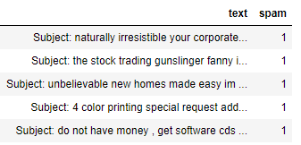
Now, we can print the top 5 rows of our dataframe
data_frame.head()
The below table shows the text and spam, as two columns, the text feature is the descriptive feature which contains the email: subject and body content. The spam column contains two ham and spam class labels, where 0 refers to ham and 1 refers to spam
# Let's get the length of the messages
data_frame['length'] = data_frame['text'].apply(len)
data_frame['length'].max()
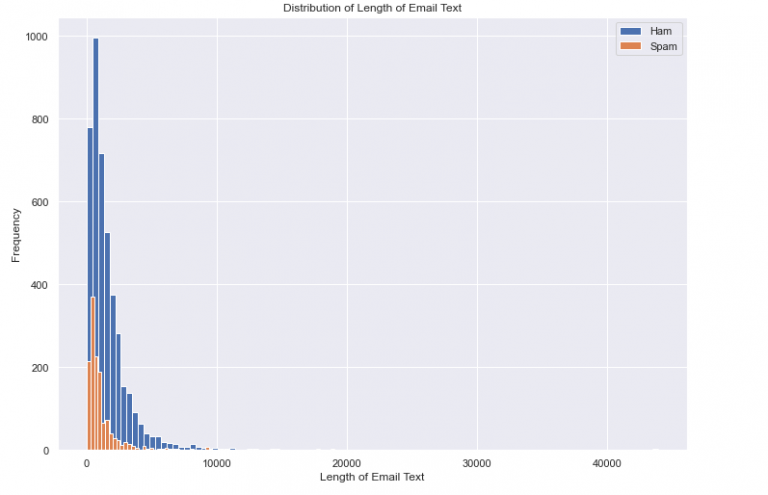
#Length of characters for ham emails is more as compared to spam emails
sns.set(rc={'figure.figsize':(11.7,8.27)})
ham_messages_length =  data_frame[data_frame['spam']==0]
spam_messages_length =  data_frame[data_frame['spam']==1]

ham_messages_length['length'].plot(bins=100, kind='hist',label = 'Ham')
spam_messages_length['length'].plot(bins=100, kind='hist',label = 'Spam')

plt.title('Distribution of Length of Email Text')
plt.xlabel('Length of Email Text')
plt.legend()
The below code snippet separates the ham and spam emails and counts the max word length used in any spam or ham email. For ham email, the maximum number of words used in an email is 8479 and for spam email, the maximum word used is 6131
#data_frame['spam']==0
data_frame[data_frame['spam']==0].text.values

ham_words_length = [len(word_tokenize(title)) for title in data_frame[data_frame['spam']==0].text.values]
spam_words_length = [len(word_tokenize(title)) for title in data_frame[data_frame['spam']==1].text.values]
print(max(ham_words_length))
print(max(spam_words_length))
8479
6131
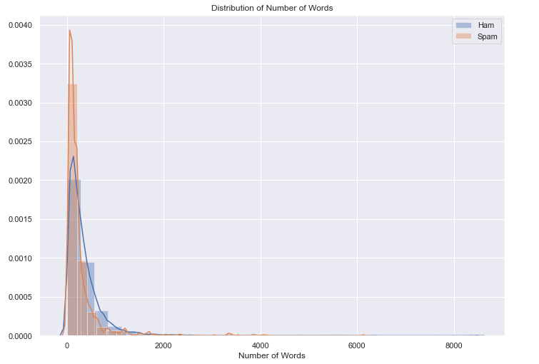
From the above code snippet, we get the number of words for each document for the spam and ham category. Now in the below code snippet, we plotted a histogram that shows the distribution of the number of words.
#There is spike in spam emails with less number of words
#Even when our dataset include 24 percent of spam emails out of total emails-
#Looks like Spam emails have less words as compared to ham emails
sns.set(rc={'figure.figsize':(11.7,8.27)})
ax = sns.distplot(ham_words_length, norm_hist = True, bins = 30, label = 'Ham')
ax = sns.distplot(spam_words_length, norm_hist = True, bins = 30, label = 'Spam')
#ham_words_length.plot(bins=100, kind='hist',label = 'Ham')
#spam_words_length.plot(bins=100, kind='hist',label = 'Spam')


plt.title('Distribution of Number of Words')
plt.xlabel('Number of Words')
plt.legend()

plt.show()
Then we plotted histogram for distribution of mean word length used in spam and ham category using the below code snippet.
def mean_word_length(x):
    word_lengths = np.array([])
    for word in word_tokenize(x):
        word_lengths = np.append(word_lengths, len(word))
    return word_lengths.mean()

ham_meanword_length = data_frame[data_frame['spam']==0].text.apply(mean_word_length)
spam_meanword_length = data_frame[data_frame['spam']==1].text.apply(mean_word_length)


sns.distplot(ham_meanword_length, norm_hist = True, bins = 30, label = 'Ham')
sns.distplot(spam_meanword_length , norm_hist = True, bins = 30, label = 'Spam')
plt.title('Distribution of Mean Word Length')
plt.xlabel('Mean Word Length')
plt.legend()
plt.show()

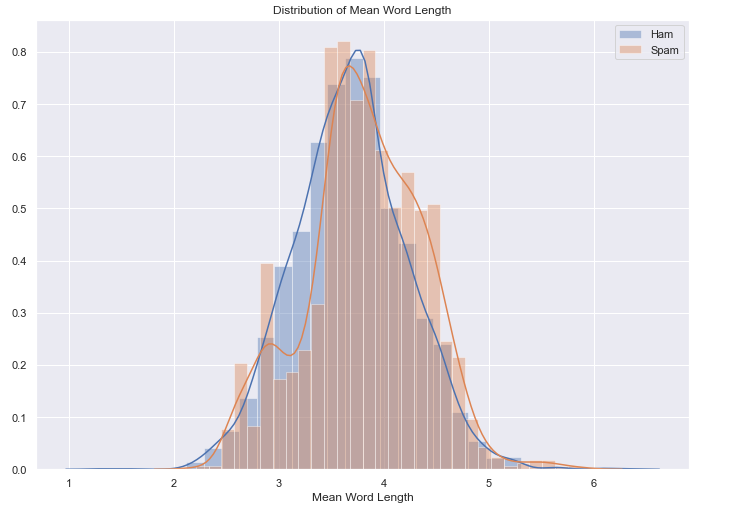
#There is not a significant difference for the length of words used by ham and spam emails
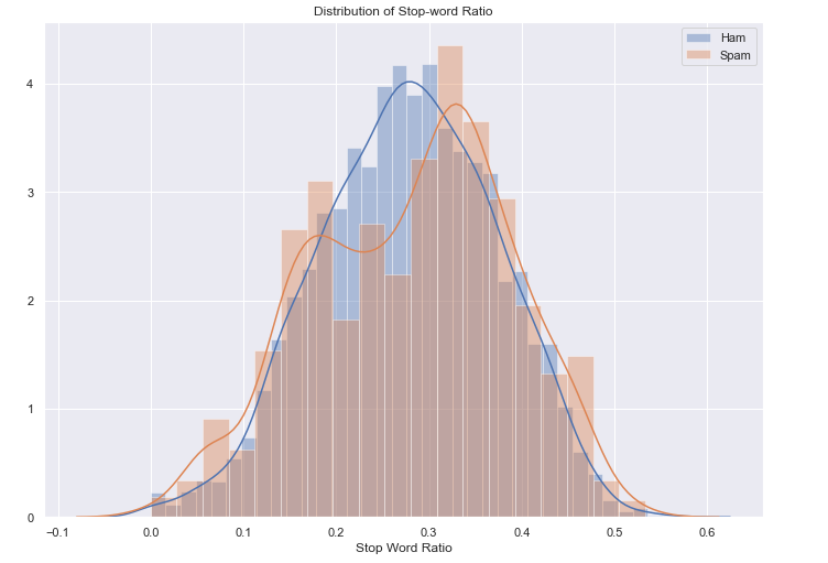
Then we plotted histogram for distribution of stop word ratio in each mail used in spam and ham category using the below code snippet.
#Checking ratio of stop words
#Both spam and ham email contain stopwords
#All Spam emails contain stop words with a mean of 0.281
#All Ham emails contain stop words with a mean of 0.278
#But we can see from the graph, spam email contain high stop words ratio as compared to ham emails.
from nltk.corpus import stopwords
stop_words = set(stopwords.words('english'))


def stop_words_ratio(x):
    num_total_words = 0
    num_stop_words = 0
    for word in word_tokenize(x):
        if word in stop_words:
            num_stop_words += 1
        num_total_words += 1
    return num_stop_words/num_total_words


ham_stopwords = data_frame[data_frame['spam']==0].text.apply(stop_words_ratio)
spam_stopwords = data_frame[data_frame['spam']==1].text.apply(stop_words_ratio)


sns.distplot(ham_stopwords, norm_hist = True, label = 'Ham')
sns.distplot(spam_stopwords,  label = 'Spam')

print('Ham Mean: {:.3f}'.format(ham_stopwords.values.mean()))
print('Spam Mean: {:.3f}'.format(spam_stopwords.values.mean()))
plt.title('Distribution of Stop-word Ratio')
plt.xlabel('Stop Word Ratio')
plt.legend()
Ham Mean: 0.278
Spam Mean: 0.281
spam_stopwords
0       0.230769
1       0.277778
2       0.397727
3       0.191919
4       0.396226
          ...
1363    0.342105
1364    0.365854
1365    0.437500
1366    0.446809
1367    0.320024
Name: text, Length: 1368, dtype: float64
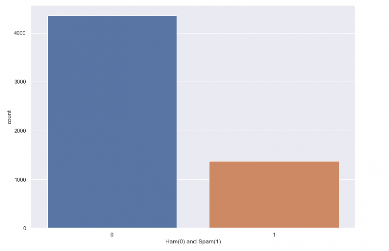
The next code snippet shows the histogram for the count of ham and spam emails present in our document and also calculate the percentage of the number of spam and ham email present.
# Let's divide the messages into spam and ham
ham = data_frame[data_frame['spam']==0]
spam = data_frame[data_frame['spam']==1]
spam['length'].plot(bins=60, kind='hist')
ham['length'].plot(bins=60, kind='hist')
data_frame['Ham(0) and Spam(1)'] = data_frame['spam']
print( 'Spam percentage =', (len(spam) / len(data_frame) )*100,"%")
print( 'Ham percentage =', (len(ham) / len(data_frame) )*100,"%")
sns.countplot(data_frame['Ham(0) and Spam(1)'], label = "Count")
Spam percentage = 23.88268156424581 %
Ham percentage = 76.11731843575419 %
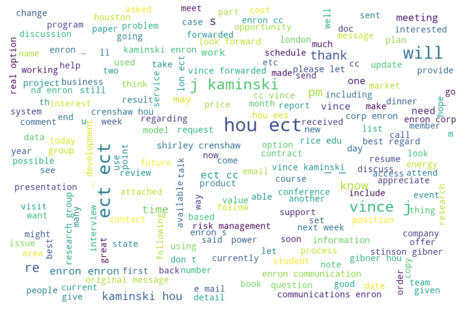
Now, we will generate a word cloud for both ham and spam emails separately using the below code. First, it creates the object for a child class generate word cloud then calling the function word cloud ham() which take two arguments, column and image filename need to be generated for the word cloud.
word_cloud_obj = generate_word_cloud()
word_cloud_obj.word_cloud(ham["text"], "ham_word_cloud.png")
word_cloud_obj.word_cloud(spam["text"], "spam_word_cloud.png")
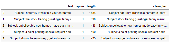
After generating word cloud, we need to perform data cleaning steps. In the below code snippet, we need to first create an object on child class data_cleaning and then calling function apply_to_column using the created object. The function takes input as text feature which is a data frame column and returns the processed data frame and stored in
another column named clean_text.
data_clean_obj = data_cleaning()
data_frame['clean_text'] = data_clean_obj.apply_to_column(data_frame['text'])
data_frame.head()
We can now check the additional columns created by using the pandas head function on the data frame
data_obj.data_frame.head()
data_obj.write_to_csvfile("processed_file.csv")
Now applying countvectorizer on the processed data column clean text. It first creates an object for child class apply_embedding_and_model. Then calling the function apply count vector which takes the column input and returns the countvectorizer sparse matrix.
#APPLY COUNT VECTORIZER TO OUR MESSAGES LIST

# Define the cleaning pipeline we defined earlier
#vectorizer = CountVectorizer()
cv_object = apply_embeddding_and_model()
spamham_countvectorizer = cv_object.apply_count_vector(data_frame['clean_text'])
Now we need to separate descriptive and target features from our data set.
#Separating Descriptive and Target Feature
X = spamham_countvectorizer
label = data_frame['spam'].values
y = label
This function will implement the email spam classification using naive bayes. Now, we need to call the function apply_naive_bayes using the object created for child class apply_embedding_and_model.
cv_object.apply_naive_bayes(X,y)
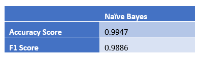
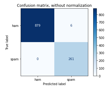
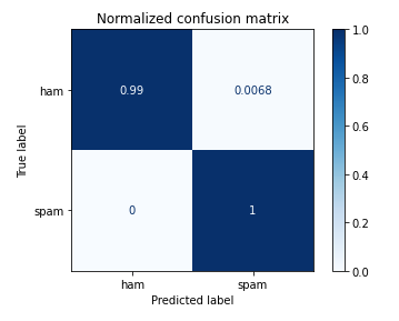
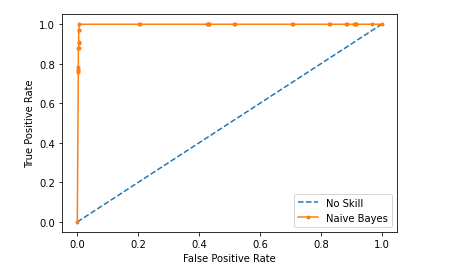
The apply_naive_bayes function performs the below mention jobs.
• It split the training and test set to 80% and 20% ratio.
• Apply the Naive Bayes on training data.
• Predict the outcome of the test dataset.
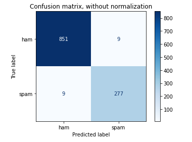
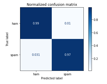
• Calculate confusion matrix without normalization and with normalization.
• Calculate Accuracy, F1, Recall, and Precision.
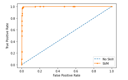
• Plot ROC curve.
Now, we need to call the function apply_svm using the object created for child class apply_embedding_and_model
This function will implement the email spam classification using svm.Now, we need to call the function apply_svm using the object created for child class apply_embedding_and_model
cv_object.apply_svm(X,y)
The apply_svm function performs the below mention jobs.
• It split the training and test set to 80% and 20% ratio.
• Apply the Naive Bayes on training data.
• Predict the outcome of the test dataset.
• Calculate confusion matrix without normalization and with normalization.
• Calculate Accuracy, F1, Recall, and Precision.
• Plot ROC curve.
Results
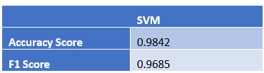
Comparing both Naïve Bayes and SVM, I found that Naïve Bayes has 1% improvement over the SVM model when the result compared to the email spam classification test dataset.
Do not forget to read the email spam classification project report to have a complete understanding using the CRISP-DM approach.
Following are the links and references regarding email spam detection and classification research papers
• Basu, Atreya Watters, Carolyn Author, Michael. (2003). Support Vector Machines for Text Categorization. 103. 10.1109/HICSS.2003.1174243.
• Zhang, Wei Gao, Feng. (2011). An Improvement to Naive Bayes for Text Classification. Procedia Engineering. 15. 2160-2164. 10.1016/j.proeng.2011.08.404.
• https://www.kaggle.com/venky73/spam-mails-dataset