Email Spam Classification Project Report

Email Spam classification Project Report: CRISP-DM

The project titled “Email Spam classification” is implemented using the CRISP-DM methodology. You will get to know Business understanding, Data Understanding (Data Description and Exploration), Data Preparation, Modelling, and Evaluation steps. Project is implemented using Python class object-based style. Email spam detection is done using machine learning algorithms Naive Bayes and SVM (Support vector machines). Further, it shows the complete program flow for Python-based email spam classifier implementation such as Data Retrieval Flow, Data Visualization Flow, Data Preparation Flow, Modeling, and Evaluation Flow. Also, including the section regarding Data ethics. In case you want to understand and demystify the python code using a top-down approach visit the following link email spam classification and detection python code.

Business Understanding

Most of us consider spam emails as one which is annoying and repetitively used for purpose of advertisement and brand promotion. We keep on blocking such email-ids but it is of no use as spam emails are still prevalent. Some major categories of spam emails that are causing great risk to security, such as fraudulent e-mails, identify theft, hacking, viruses, and malware. In order to deal with spam emails, we need to build a robust real-time email spam classifier that can efficiently and correctly flag the incoming mail spam, if it is a spam message or looks like a spam message. The latter will further help to build an Anti-Spam Filter.

Google and other email services are providing utility for flagging email spam but are still in the infancy stage and need regular feedback from the end-user. Also, popular email services such as Gmail, Yandex, yahoo mail, etc provide basic services as free to the end-user and that of course comes with EULA. There is a great scope in building email spam classifiers, as the private companies run their own email servers and want them to be more secure because of the confidential data, in such cases email spam classifier solutions can be provided to such companies.

Data understanding

The email spam classifier focuses on either header, subject, and content of the email. In this project, we are focusing mainly on the subject and content of the email.

To download the email spam classification dataset files and complete code and visit the link email spam detection and classification project GitHub repository.

Data Description

The dataset contains two columns. The total corpus of 5728 documents. The descriptive feature consists of text. The target feature consists of two classes ham and spam, the column name is spam. The classes are labeled for each document in the data set and represent our target feature with a binary string-type alphabet of {ham; spam}. Classes are further mapped to integer 0 (ham) and 1 (spam).

 

 

Data exploration

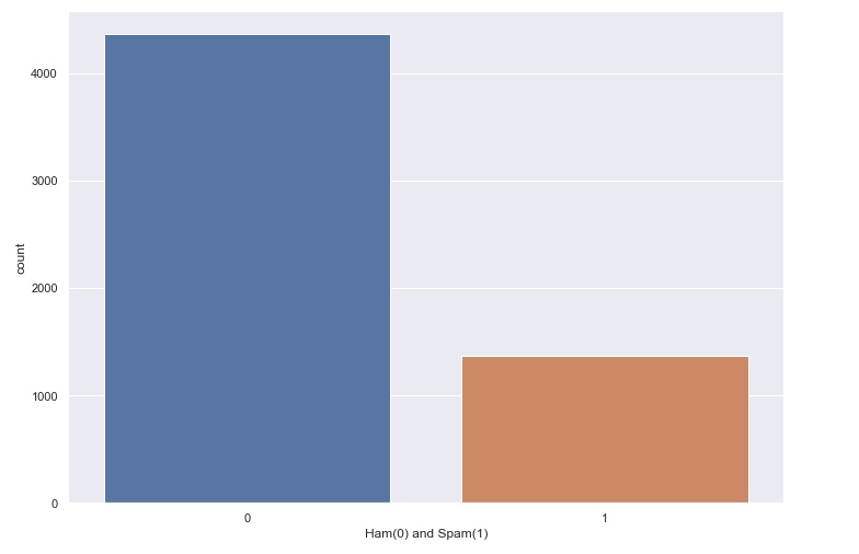
Spam email percentage in the dataset = 23.88268156424581 %

Ham email percentage in the dataset = 76.11731843575419 %

The bar graph given below depicts the percentage of Ham and Spam emails in the given dataset. The blue bar represents the count of ham emails and the red bar shows the count of spam emails in the dataset.

 

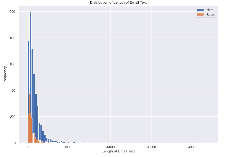
Plotting histogram for email text length of spam vs ham

Both ham and spam emails are more prevalent for shorter lengths. As spam emails are 24% of the whole data, so its obvious frequency of spam emails is less as compared to ham emails.

 

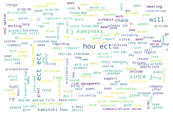
Word cloud for ham emails

 

 

 

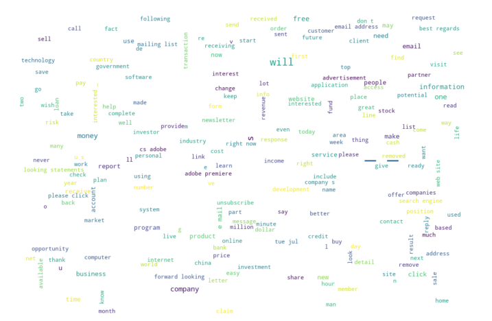
Word cloud for spam emails

 

 

 

 

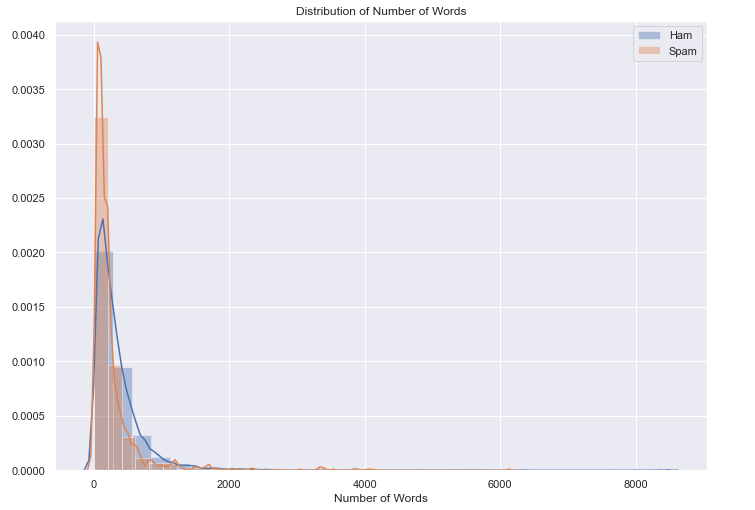
Distribution of the number of words: From the below figure we can see that, there is a spike in spam emails with a smaller number of words, even when our dataset includes 24 percent of spam emails out of total emails.

 

 

 

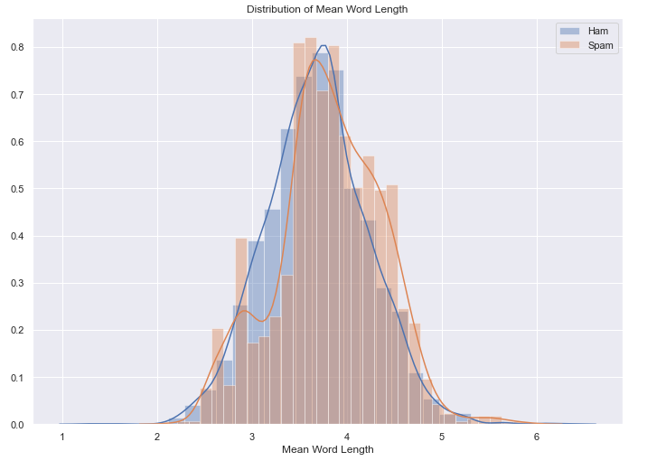
Exploring mean word length: There is not a significant difference in the length of words used by ham and spam emails.

 

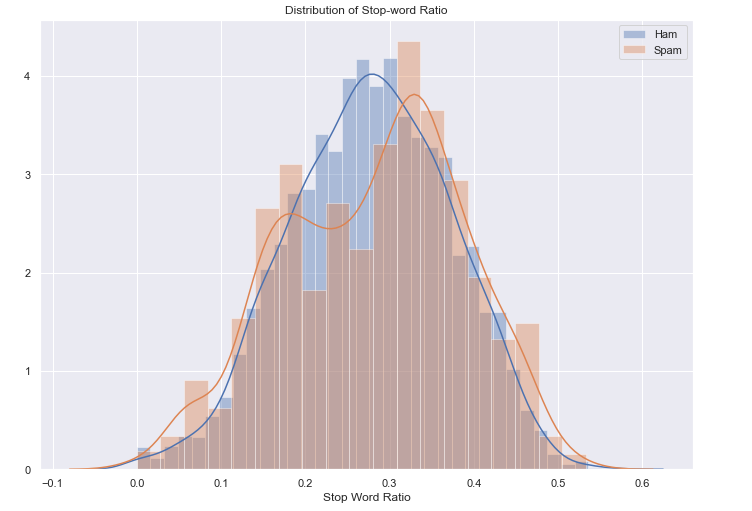
Distribution of Stop-word ratio:

• All Spam emails contain stop words with a mean of 0.281
• All Ham emails contain stop words with a mean of 0.278
• But we can see from the graph, spam email contains high stop words ratio as compared to ham emails.

 

 

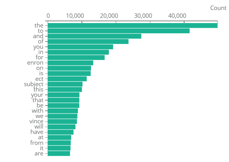
Most Frequent word analysis using stop words: 

 

 

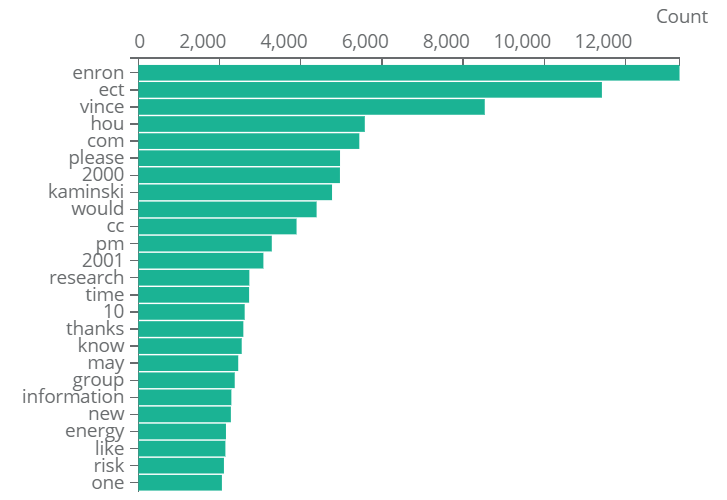
Most Frequent word analysis without using stop words: 

 

 

Data preparation

The following steps we used for data preparation.

• Identifying Missing values.
• Converting all text to lower case.
• Performing tokenization.
• Removing Stop words.
• Labelling classes: ham/spam: {0;1}
• Splitting Train and Test Data: 80% and 20%.

 

Modeling

Feature representation: Using word embedding technique CountVectorizer.

Models used: Naive Bayes and SVM. Email spam classification done using traditional machine learning techniques comprise Baive Bayes and SVM (support vector machines), due to not having sufficient hardware resources, takes less time to train. Also, not opting for neural algorithms due to less data and computing resources.

Reason for choosing SVM and Naïve Bayes: Both are good at handling large number of features; in the case of text classification each word is a feature and we have thousands of words based on the vocabulary of the corpus.  SVM works best with high dimensional data, a vocabulary with 1000 words means each text in the corpus will be represented with a vector of 1000 dimension.

When we have a sufficient number of features, both SVM and Naïve Bayes can work with less data as well.

Naïve Bayes does not suffer from curse-of-dimensionality because it treats all features as independent of one another. Also, one of the benefits of features being independent is: For example, most spam emails contain words such as money and investment, etc, but it is not necessary that all the mails containing both words money and investment are considered to be spam.

Feature representation: Word embeddings can be broadly classified into two categories: Frequency and prediction-based. I have chosen a count vector that shows the count of occurrence of a feature in the given document, thus it is a matrix of document vs vocabulary (containing all the features as a column).

In our case, the size of the Count vector matrix is 5728 x 20114, where 5728 represents the number of documents in the corpus and 20114 represents the number of features in the vocabulary.

Splitting Training and Testing Data: Splitting the data into training and test datasets, where training data contains 80 percent and test data contains 20 percent.

Applying model SVM and Naïve Bayes: I trained the model for both SVM and Naive without tuning hyperparameters as I got results with default parameter settings.

 

Evaluation

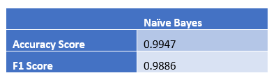
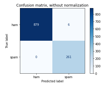
Naïve Bayes Result on Test dataset:

 

 

Confusion matrix for Naïve Bayes without normalization

 

Confusion matrix for Naïve Bayes with normalization

 

 

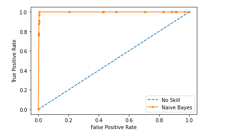
Naïve Bayes ROC Curve

 

 

 

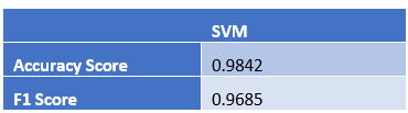
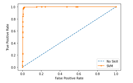
SVM Result on Test data set

 

 

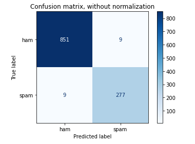
Confusion matrix for SVM without normalization

 

 

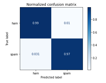
Confusion matrix for SVM with normalization

 

ROC curve for SVM model

 

Results

Comparing both Naïve Bayes and SVM, I found that Naïve Bayes has 1% improvement over the SVM model when the result compared to test data set.

 

Deployment

A supportive tool using a browser plugin or API can be built for companies running their own email servers so that they can keep a check on emails and can identify and flag spam emails. Such a supportive tool can be used in conjunction with existing email service providers as well.

Data Ethics

There are many ethical and legal issues that can really take a toll on designing such models. Bank and Investment organizations that run their own email servers have confidential emails and identity information related to customers. Using such confidential information for the predictive analysis required to safeguard the client data with the care of a professional fiduciary. Need to protect the customer data from both intentional and inadvertent disclosure, also protecting it from misuse.

Also, while implementation it is possible to generate false positive, which means the emails which are not spam fall into the spam category. An important piece of information a company can miss if the user’s legit email is marked as spam. A client or user who is a loyal customer, his email can be marked spam, which is an ethical issue.

Email Spam Classifier: Object-oriented model with program flow

 

Object-oriented model for the Project.

We have one parent class and three child class which inherit data and functions from the parent class.
Parent class: data_read_write Child class: generate_word_cloud |data_cleaning| apply_ embedding_and_model

 

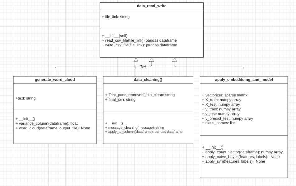
Program Flow

 

We have four classes in total. One is the parent and three child classes.
• Parent class: data_read_write
• Child class: generate_word_cloud
• Child class: data_cleaning
• Child class: apply_embedding_and_model

 

Data Retrieval Flow

The program flow also shows how we retrieved the data, we have used CSV file, which we directly downloaded from the Kaggle email spam data set link. The below steps mention how we read and done operation on csv file using pandas.

Creating object on the parent class: data_read_write

data_obj = data_read_write("emails.csv")

 

We create an object by initializing it using the dataset file emails.csv which is passed to the constructor. It will read the name of the file and store it in file_link variable which is a string type and return the object reference. We can now
read the CSV file by calling read_csv_file() function defined in our parent class data_read_write by accessing it through the object. The function will return the content of the file as pandas dataframe

data_frame = data_obj.read_csv_file()

 

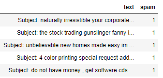
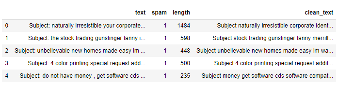
Now, we can print the top 5 rows of our dataframe

data_frame.head()

 

The below table shows the text and spam, as two columns, the text feature is the descriptive feature which contains the email: subject and body content. The spam column contains two ham and spam class labels, where 0 refers to ham and 1 refers to spam

Data Visualization Flow

The below code snippet separates the ham and spam emails and counts the max word length used in any spam or ham
email. For ham email, the maximum number of words used in an email is 8479 and for spam email, the maximum word used is 6131

#data_frame['spam']==0
data_frame[data_frame['spam']==0].text.values

ham_words_length = [len(word_tokenize(title)) for title in data_frame[data_frame['spam']==0].text.values]
spam_words_length = [len(word_tokenize(title)) for title in data_frame[data_frame['spam']==1].text.values]
print(max(ham_words_length))
print(max(spam_words_length))

 

From the above code snippet, we get the number of words for each document for the spam and ham category. Now in the below code snippet, we plotted a histogram that shows the distribution of the number of words.

#There is spike in spam emails with less number of words
#Even when our dataset include 24 percent of spam emails out of total emails-
#Looks like Spam emails have less words as compared to ham emails
sns.set(rc={'figure.figsize':(11.7,8.27)})
ax = sns.distplot(ham_words_length, norm_hist = True, bins = 30, label = 'Ham')
ax = sns.distplot(spam_words_length, norm_hist = True, bins = 30, label = 'Spam')
#ham_words_length.plot(bins=100, kind='hist',label = 'Ham') 
#spam_words_length.plot(bins=100, kind='hist',label = 'Spam')


plt.title('Distribution of Number of Words')
plt.xlabel('Number of Words')
plt.legend()
                       
plt.show()

 

Then we plotted histogram for distribution of mean word length used in spam and ham category using the below code snippet.

def mean_word_length(x):
    word_lengths = np.array([])
    for word in word_tokenize(x):
        word_lengths = np.append(word_lengths, len(word))
    return word_lengths.mean()

ham_meanword_length = data_frame[data_frame['spam']==0].text.apply(mean_word_length)
spam_meanword_length = data_frame[data_frame['spam']==1].text.apply(mean_word_length)


sns.distplot(ham_meanword_length, norm_hist = True, bins = 30, label = 'Ham')
sns.distplot(spam_meanword_length , norm_hist = True, bins = 30, label = 'Spam')
plt.title('Distribution of Mean Word Length')
plt.xlabel('Mean Word Length')
plt.legend()
plt.show()

#There is not a significant difference for the length of words used by ham and spam emails

 

Then we plotted histogram for distribution of stop word ratio in each mail used in spam and ham category using the below code snippet.

#Checking ratio of stop words
#Both spam and ham email contain stopwords
#All Spam emails contain stop words with a mean of 0.281
#All Ham emails contain stop words with a mean of 0.278
#But we can see from the graph, spam email contain high stop words ratio as compared to ham emails.
from nltk.corpus import stopwords
stop_words = set(stopwords.words('english'))
    
    
def stop_words_ratio(x):
    num_total_words = 0
    num_stop_words = 0
    for word in word_tokenize(x):
        if word in stop_words:
            num_stop_words += 1
        num_total_words += 1 
    return num_stop_words/num_total_words


ham_stopwords = data_frame[data_frame['spam']==0].text.apply(stop_words_ratio)
spam_stopwords = data_frame[data_frame['spam']==1].text.apply(stop_words_ratio)


sns.distplot(ham_stopwords, norm_hist = True, label = 'Ham')
sns.distplot(spam_stopwords,  label = 'Spam')

print('Ham Mean: {:.3f}'.format(ham_stopwords.values.mean()))
print('Spam Mean: {:.3f}'.format(spam_stopwords.values.mean()))
plt.title('Distribution of Stop-word Ratio')
plt.xlabel('Stop Word Ratio')
plt.legend()

 

The next code snippet shows the histogram for the count of ham and spam emails present in our document and also calculate the percentage of the number of spam and ham email present.

# Let's divide the messages into spam and ham
ham = data_frame[data_frame['spam']==0]
spam = data_frame[data_frame['spam']==1]
spam['length'].plot(bins=60, kind='hist') 
ham['length'].plot(bins=60, kind='hist') 
data_frame['Ham(0) and Spam(1)'] = data_frame['spam']
print( 'Spam percentage =', (len(spam) / len(data_frame) )*100,"%")
print( 'Ham percentage =', (len(ham) / len(data_frame) )*100,"%")
sns.countplot(data_frame['Ham(0) and Spam(1)'], label = "Count")

 

Spam percentage = 23.88268156424581 %
Ham percentage = 76.11731843575419 %

 

Now, we will generate a word cloud for both ham and spam emails separately using the below code. First, it creates the object for a child class generate word cloud then calling the function word cloud ham() which take two arguments, column and image filename need to be generated for the word cloud.

word_cloud_obj = generate_word_cloud()
word_cloud_obj.word_cloud(ham["text"], "ham_word_cloud.png")
word_cloud_obj.word_cloud(spam["text"], "spam_word_cloud.png")

 

Below can see a complete class, data, and methods of the child class generate_word_cloud child class generate_word_cloud

#Child Class for Data_read_write
class generate_word_cloud(data_read_write):
    def __init__(self):
        pass
    #Child own Function
    def variance_column(self, data):
        return variance(data)
    #Polymorphism
    def word_cloud(self, data_frame_column, output_image_file):
        text = " ".join(review for review in data_frame_column)
        stopwords = set(STOPWORDS)
        stopwords.update(["subject"])
        wordcloud = WordCloud(width = 1200, height = 800, stopwords=stopwords, max_font_size = 50, 
                              margin=0, background_color = "white").generate(text)
        plt.imshow(wordcloud, interpolation='bilinear')
        plt.axis("off")
        plt.show()
        wordcloud.to_file(output_image_file)
        return

 

Data Preparation Flow

After generating word cloud, we need to perform data cleaning steps. In the below code snippet, we need to first create an object on child class data_cleaning and then calling function apply_to_column using the created object. The function takes input as text feature which is a data frame column and returns the processed data frame, and stored in
another column named clean_text.

data_clean_obj = data_cleaning()
data_frame['clean_text'] = data_clean_obj.apply_to_column(data_frame['text'])

 

We can see that the data_cleaning class consists of two methods apply_to_column which calls another function message_cleaning which further removes stop words, remove punctuation, and do necessary data processing steps.

#Child Class for Data_read_write
class data_cleaning(data_read_write):
    def __init__(self):
        pass
    def message_cleaning(self, message):
            Test_punc_removed = [char for char in message if char not in string.punctuation]
            Test_punc_removed_join = ''.join(Test_punc_removed)
            Test_punc_removed_join_clean = [word for word in Test_punc_removed_join.split() 
                                            if word.lower() not in stopwords.words('english')]
            final_join = ' '.join(Test_punc_removed_join_clean)
            return final_join
    
        
    def apply_to_column(self, data_column_text):
        data_processed = data_column_text.apply(self.message_cleaning)
        return data_processed

 

We can now check the additional columns created by using the pandas head function on the data frame

data_obj.data_frame.head()

 

 

 

Modeling and Evaluation Flow

Then applying countvectorizer on the processed data column clean text. It first creates an object for child class apply_embedding_and_model. Then calling the function apply count vector which takes the column input and returns the countvectorizer sparse matrix.

 

#APPLY COUNT VECTORIZER TO OUR MESSAGES LIST

# Define the cleaning pipeline we defined earlier
#vectorizer = CountVectorizer()
cv_object = apply_embeddding_and_model()
spamham_countvectorizer = cv_object.apply_count_vector(data_frame['clean_text'])

 

Now we need to separate descriptive and target features from our data set.

#Separating Descriptive and Target Feature 
X = spamham_countvectorizer
label = data_frame['spam'].values
y = label

 

Now, we need to call the function apply_naive_bayes using the object created for child class apply_embedding_and_model

cv_object.apply_naive_bayes(X,y)

 

The apply_naive_bayes function performs the below mention jobs.
• It split the training and test set to 80% and 20% ratio.
• Apply the Naive Bayes on training data.
• Predict the outcome of the test dataset.
• Calculate confusion matrix without normalization and with normalization.
• Calculate Accuracy, F1, Recall, and Precision.
• Plot ROC curve.

Now, we need to call the function apply_svm using the object created for child class apply_embedding_and_model

cv_object.apply_svm(X,y)

 

The apply_svm function performs the below mention jobs.
• It split the training and test set to 80% and 20% ratio.
• Apply the Naive Bayes on training data.
• Predict the outcome of the test dataset.
• Calculate confusion matrix without normalization and with normalization.
• Calculate Accuracy, F1, Recall, and Precision.
• Plot ROC curve.

Given below is the code snippet for child class apply embedding and model which shows all the data variables and three methods used in the class.

#Child Class for Data_read_write
class apply_embeddding_and_model(data_read_write):
    def __init__(self):
        pass
    def apply_count_vector(self, v_data_column):
        vectorizer = CountVectorizer(min_df=2,analyzer = "word",tokenizer = None,preprocessor = None,stop_words = None)
        return vectorizer.fit_transform(v_data_column)
        
    def apply_naive_bayes(self, X, y):
        #DIVIDE THE DATA INTO TRAINING AND TESTING PRIOR TO TRAINING
        X_train, X_test, y_train, y_test = train_test_split(X, y, test_size=0.2)
        #Training model
        NB_classifier = MultinomialNB()
        NB_classifier.fit(X_train, y_train)
        # Predicting the Test set results
        y_predict_test = NB_classifier.predict(X_test)
        cm = confusion_matrix(y_test, y_predict_test)
        #sns.heatmap(cm, annot=True)
        #Evaluating Model
        print(classification_report(y_test, y_predict_test))
        print("test set")
        print("\nAccuracy Score: " + str(metrics.accuracy_score(y_test, y_predict_test)))
        print("F1 Score: " + str(metrics.f1_score(y_test, y_predict_test)))
        print("Recall: " + str(metrics.recall_score(y_test, y_predict_test)))
        print("Precision: " + str(metrics.precision_score(y_test, y_predict_test)))
        
        class_names = ['ham', 'spam']
        titles_options = [("Confusion matrix, without normalization", None),
                  ("Normalized confusion matrix", 'true')]
        for title, normalize in titles_options:
            disp = plot_confusion_matrix(NB_classifier, X_test, y_test,
                                 display_labels=class_names,
                                 cmap=plt.cm.Blues,
                                 normalize=normalize)
            disp.ax_.set_title(title)
            print(title)
            print(disp.confusion_matrix)
        plt.show()
         # generate a no skill prediction (majority class)
        ns_probs = [0 for _ in range(len(y_test))]
        # predict probabilities
        lr_probs = NB_classifier.predict_proba(X_test)
        # keep probabilities for the positive outcome only
        lr_probs = lr_probs[:, 1]
        # calculate scores
        ns_auc = roc_auc_score(y_test, ns_probs)
        lr_auc = roc_auc_score(y_test, lr_probs)
        # summarize scores
        print('No Skill: ROC AUC=%.3f' % (ns_auc))
        print('Naive Bayes: ROC AUC=%.3f' % (lr_auc))
        # calculate roc curves
        ns_fpr, ns_tpr, _ = roc_curve(y_test, ns_probs)
        lr_fpr, lr_tpr, _ = roc_curve(y_test, lr_probs)
        # plot the roc curve for the model
        pyplot.plot(ns_fpr, ns_tpr, linestyle='--', label='No Skill')
        pyplot.plot(lr_fpr, lr_tpr, marker='.', label='Naive Bayes')
        # axis labels
        pyplot.xlabel('False Positive Rate')
        pyplot.ylabel('True Positive Rate')
        # show the legend
        pyplot.legend()
        # show the plot
        pyplot.show()
        return
    def apply_svm(self, X, y):
        #DIVIDE THE DATA INTO TRAINING AND TESTING PRIOR TO TRAINING
        X_train, X_test, y_train, y_test = train_test_split(X, y, test_size=0.2)
        #Training model
        #'linear', 'poly', 'rbf'
        params = {'kernel': 'linear', 'C': 2, 'gamma': 1}
        svm_cv = svm.SVC(C=params['C'], kernel=params['kernel'], gamma=params['gamma'], probability=True)
        svm_cv.fit(X_train, y_train)
        # Predicting the Test set results
        y_predict_test = svm_cv.predict(X_test)
        cm = confusion_matrix(y_test, y_predict_test)
        #sns.heatmap(cm, annot=True)
        #Evaluating Model
        print(classification_report(y_test, y_predict_test))
        print("test set")

        print("\nAccuracy Score: " + str(metrics.accuracy_score(y_test, y_predict_test)))
        print("F1 Score: " + str(metrics.f1_score(y_test, y_predict_test)))
        print("Recall: " + str(metrics.recall_score(y_test, y_predict_test)))
        print("Precision: " + str(metrics.precision_score(y_test, y_predict_test)))
        
        class_names = ['ham', 'spam']
        titles_options = [("Confusion matrix, without normalization", None),
                  ("Normalized confusion matrix", 'true')]
        for title, normalize in titles_options:
            disp = plot_confusion_matrix(svm_cv, X_test, y_test,
                                 display_labels=class_names,
                                 cmap=plt.cm.Blues,
                                 normalize=normalize)
            disp.ax_.set_title(title)
            print(title)
            print(disp.confusion_matrix)
        plt.show()
        
        # generate a no skill prediction (majority class)
        ns_probs = [0 for _ in range(len(y_test))]
        # predict probabilities
        lr_probs = svm_cv.predict_proba(X_test)
        # keep probabilities for the positive outcome only
        lr_probs = lr_probs[:, 1]
        # calculate scores
        ns_auc = roc_auc_score(y_test, ns_probs)
        lr_auc = roc_auc_score(y_test, lr_probs)
        # summarize scores
        print('No Skill: ROC AUC=%.3f' % (ns_auc))
        print('SVM: ROC AUC=%.3f' % (lr_auc))
        # calculate roc curves
        ns_fpr, ns_tpr, _ = roc_curve(y_test, ns_probs)
        lr_fpr, lr_tpr, _ = roc_curve(y_test, lr_probs)
        # plot the roc curve for the model
        pyplot.plot(ns_fpr, ns_tpr, linestyle='--', label='No Skill')
        pyplot.plot(lr_fpr, lr_tpr, marker='.', label='SVM')
        # axis labels
        pyplot.xlabel('False Positive Rate')
        pyplot.ylabel('True Positive Rate')
        # show the legend
        pyplot.legend()
        # show the plot
        pyplot.show()
        return

 

Do not forget to read the email spam detection and classification python code to have a complete understanding of the code in a top-down. To download the complete code visit the link email spam detection and classification project GitHub repository.

Following are the links and references regarding email spam detection research papers

• Basu, Atreya Watters, Carolyn Author, Michael. (2003). Support Vector Machines for Text     Categorization. 103. 10.1109/HICSS.2003.1174243.
• Zhang, Wei Gao, Feng. (2011). An Improvement to Naive Bayes for Text Classification.       Procedia Engineering. 15. 2160-2164. 10.1016/j.proeng.2011.08.404.
• https://www.kaggle.com/venky73/spam-mails-dataset